Trade and the flag:
integration and conflict in 19th and
early 20th century
deglobalization
Chris
Chase-Dunn, Anders Carlson, Chris Schmitt, Shoon Lio,
Richard
Niemeyer and Robert A. Hanneman
Institute for Research on World-Systems
University
of California-Riverside,
To be presented at the Section on Peace, War, and Social Conflict Roundtable, Fri, Aug 11 - 2:30pm - 3:25pm, Annual meeting of the American Sociological Association, Montreal. Draft v.8-9-06; 7470 words
IROWS
Working Paper #19 https://irows.ucr.edu/papers/irows19/irows19.htm
Abstract:
The density and contours of
networks of transnational and international economic integration are
hypothesized by many theorists to be causally related to the patterns of
cooperation and conflict. [1]
The usual notion is that trade creates ties of symmetrical interdependence,
which are likely to inhibit conflict. We seek to test this hypothesis in the
19th and early 20th century run-up to World War I. We examine the
relationship between the structure of conflict and the contours of trade ties
during the 19th century wave of globalization and deglobalization. How were the international trade ties related
to the patterns of conflict and alliance that emerged during World War I?
Waves of Globalization
Over the past few
decades, there has been a surge of interest in the relationship between
globalization and political conflict in the interstate system. Most of the theorists
of the global capitalism school contend that beginning with the 1960s and
1970s, the world of national economies became transformed into a transnational
and global political economy (e.g. Sklair 2001). Scholars using the world-systems perspective
contend that the world-system of capitalism has been importantly transnational
for hundreds of years and that globalization in the sense of the expansion and
intensification of large-scale intercontinental interaction networks is both an
upward trend and a cycle. There were earlier periods of rapid globalization
that were followed by periods of deglobalization in which large-scale
interactions diminished. Keynesian
national development (the global New Deal) was the predominant strategy of the
development project led by the hegemonic
Neoliberalism was
the political ideology that became hegemonic in the 1980s because the competing
core countries -
Yet, in contrast
to the global capitalism school, we argue that the old system of national
states still exists and that something like the current wave of globalization
had happened before during the decline of British hegemony in the late 19th and early 20th century.
Studies of trade globalization – the ratio of international trade to the world
GDP-- show that there was a high peak in
the 1880s, then a decline until 1900, then another small rise, and a crash in
1929, and then a rise after World War II to the present,
which is somewhat higher than the peak in 1880, but not extremely higher (see
Figure 1). Investment globalization probably followed a similar trajectory
(Chase-Dunn, et al 2002)
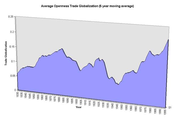
Figure 1: Waves of trade globalization (Chase-Dunn, Kawano and
Brewer 2000)
Global Elite Networks and International
Trade Links
This paper is
part of a larger project, the purpose of which is to study the contours of global
elite and international integration since 1840 and to study the relationship
between these contours of connection and the patterns of conflict that emerged
over the same time period. There have
been a significant number of theoretical and empirical works by political
scientists and sociologists that examine the effects of economic
interdependence and international conflict (McMillan 1997; Barbieri and
Schneider 1999; Barbieri 2002; Rosecrance and Thompson 2003; Maoz 2004, Maoz et al 2006, forthcoming). Various
liberal theories of globalization argue that economic integration should
decrease international conflict. [3]We
observe that these approaches should distinguish between horizontal connections
(of equality) and vertical connections (power-dependency relations). The latter
may be quite likely to produce conflict (Barbieri 2002; Rosecrance and Thompson
2003).
Contra these
perspectives, many observers have noted that interdependent connections have
not served to prevent major conflicts in the modern international system
(Thompson and Tucker 1997; Rosecrance and Thompson 2003). Both
Our larger project
consists of two parts. In the first we are using a world historical perspective
to examine the links between elite individuals, families and organizations
within each country with those same actors in other countries. This involves a
close reading of the histories of each country with attention to connections
with other countries (see Reifer and Chase-Dunn 2003; Barr et al 2006). The second part of our project (discussed here) uses
quantitative data on the interactions among nation-states to trace the changing
patterns of network connections since 1880.
This enables us to use the national network patterns to place the
information from our studies of elites in a world historical context, and to
study the congruence or lack thereof, between different kinds of international
connections. We also intend to examine the relationships between international
network structures and the patterns of conflictive relations that were so
evident in the first half of the twentieth century. We know that the
international system bifurcated into Allies and Axis states in the World Wars. Were
these conflict-alliance bloc structures related to the trade network? Did the
network of global trade become more factional in the years prior to the
outbreak of world war? And did these factions correspond with the emergent
conflict factions?
We also will eventually
use network data to compare the overall magnitude of global integration in the
nineteenth century with the magnitude and forms of integration that have
emerged since World War II.[5] The
question of global magnitudes is important because many students of
globalization have assumed that the high degree of contemporary integration of
the global capitalist class will prevent the emergence of future interimperial
rivalry and war among core states. But if there was a similarly high level of
global elite integration in the late nineteenth century this assumption may be
brought into question.
In this paper we analyze
mainly international trade relations, but international financial links are another
important dimension of global economic networks that we plan to empirically
examine in the future. Imports and exports of goods and services are much
easier to get comparable information on than flows of investment, especially
for the nineteenth century. Ideally we would like to differentiate trade flows
into goods that are more strategic and profitable vs. those that are less so.
But that is not possible on a sufficient scale for the nineteenth century.
Transnational Relations and State-centrism
The use of data on nation-states is defensible on both
theoretical and practical grounds, and should not expose us to the slings and
barbs of those who would accuse us of state-centrism. Firstly, national states
have been, and still are, important organizations within the world-system.
Transnationalism has not just arisen since 1980. There have been waves of
transnationalism and waves of nationalism since the chartered companies of the
seventeenth century organized production and distribution on a global scale. The contemporary transnational corporations
undoubtedly organize a greater portion of the total world economy than the 17th
century chartered companies did. But then and now, national states were and
remain important players on the global stage.
We may say this
without denying the perspective developed by William I. Robinson (2004) and
others on the emergence of a transnational capitalist state that reconfigures
existing national states (and international organizations) as its instruments.
Indeed, we see the emergence of a transnational state, not just in the period
since the 1980s, but since the Concert of Europe that was
The practical
reason for using data on national states is that they are the only data that
are available for most of the regions of the system over the time period that
we seek to study. As with all secondary data
analyses, we need to be chary about the ways in which the structuring of the
data by its original providers may distort our results.
Methods for Our Analysis
We adopt the
generalized strategy of measurement error modeling that is part of the
structural equations tradition. This means that instead of trying to pick the
best single empirical indicator of an underlying concept or variable, we want
to use several proxy indicators and to model the relationships among the
proxies as well as using them to estimate the true underlying values of the
variables. In practice we may not have enough data to be able to actually
employ the techniques of structural equations modeling of measurement error.
But we shall use the generalized logic of gathering multiple proxy indicators
whenever this is possible.
Because the data
are less complete in the early decades, we have a growing population of nodes
as we get closer to the present. This, and the actual changes that occurred in
country boundaries over the period studied (e.g. the break-up of the Ottoman
and Austro-Hungarian empires, etc.), mean that we have a changing set of nodes
in the network. This makes it difficult to know whether observed changes were
due to real changes in the pattern of trade ties or to the inclusion of nodes
that were formerly not included because of missing data. One approach to this
problem that we have used in earlier research is to study constant groups over time. If we find similar trends between the
constant groups and the networks that are adding (or deleting) nodes we can
infer that observed changes are not due to changes in the compared units.
Variable Construction
Trade Network Data
Much of the late 19th
century and early 20th century trade data are reported in the
country’s domestic currency, which makes cross-national comparison
impossible. There are several possible
ways to deal with this problem. One is to convert all the country currency
values into a single currency such as the pound sterling or the U.S. dollar
using currency market exchange rates.[6] There
are a number of known problems with this approach. Currency market exchange rates are set by the
competitive buying and selling of currencies during some periods, but in other
periods the exchange rates have been set by international agreements. Between
the Bretton Woods conference in 1944 and the early 1970s the U.S. dollar was
pegged to a fictitious gold standard, and other currencies were pegged to the
dollar. These regulated exchange rates can still be used to change country
currencies into dollars, but this conversion reflects a worldwide agreement to
regulate currency markets rather than a world market for money. In 1974 the
dollar and other currencies were freed to exchange in world money markets.
Another problem
is that market exchange rates reflect the activities of large currency traders,
rather than just the daily conversions of currencies carried out by people who
need to change money. The actions of currency traders are intended to make
profits by buying and selling money, and this activity does not necessarily
reflect the value of the goods and services that national economies produce.
This is why economists have tried to devise a better method for converting
currencies into a single comparable metric that is based on purchasing power in
different countries (Kravis Heston and Summers 1982). These so-called purchasing
power parity (PPP) conversion ratios are not available for the 19th
century and the whole approach has been savaged by critics (e.g. Korzeniewicz,
Stach and Patil 2004).
Another method of
making country currency values comparable is to compute a percentage using a
denominator in the same metric units (country currencies). We have the total value of exports and
imports for each country in country currency, so we could compute the
percentage of the country’s trade with a particular other trade partner. This puts the numbers into a comparable
metric: percentages. But this is not a good solution to the problem for our
purposes. It does eliminate the need to use exchange rates, but at the cost of
computing a variable that will not be useful for our purpose of examining the relative
importance of a particular trade link in the context of the larger world trade
network. Knowing that the imports of
(did we use imports, exports, both or what?)
Construction of Conflict Dyads
The
countries considered in this analysis are those that fought in World War I, those
core countries of
To quantify
the intensity of conflict between two states (dyads), we relied upon three
separate indicators: 1) the Correlates of War data set compiled by Singer and
Small measuring the number of battle deaths experienced by each country in the
WWI, and 2) the Barbieri conflict data set consisting of two ordinal measures of conflict during WWI: one
representing the level of aggression country A displayed towards country B, and
the other representing the level of aggression country B displayed towards
country A.
Interestingly, each of these data sets exhibited complimentary
weaknesses. The Correlates of War data
is useful after a country goes to war because it demonstrates how
“intensely” the country was committed to fighting as a function of the number
of its dead, but the data says nothing of the level of conflict between
countries before they go to war.
In a similar fashion, the Barbieri data does an excellent job of
demonstrating the “ramping up” processes leading up to WW1, but after the fact
it is useless in distinguishing various levels of commitment to the war once it
has begun. Further, both data sets in
isolation demonstrated very high skewness and kurtosis, making interpretation
of correlation coefficients problematic.
To
remedy both of these problems we constructed a standardized index of conflict
intensity that combined all three measures.
This was carried out by transforming the “raw” values of each data set
into standardized scores using SPSS, and summing the result. At this point we realized that by
constructing the index in this fashion, we had inadvertently reduced the
contribution of the Correlates of War data.
What was once a very large difference in intensity between “a
militarized shared border,” and, “a combined war dead of over one million
soldiers,” had now been reduced to a one or two point index difference. Also, one country’s decision to enter into the
war as an ally of another is an indicator level of (low) conflict intensity
that was not being taken into account. So we modified our conflict indicator by
doubling the weight of the contribution of the battle deaths, and also coding
for whether or not a state was an ally of another.
So as to make neutrality during WWI represent zero
conflict between a pair of states, the index was scaled so that a value of –3.16
equated to war ally, 0 equated to neutral and a value of 16 equated to the highest level of conflict intensity. We do not have a measure that takes into
account various degrees of “war ally,” so the index jumps from –3.14 to 0, and
then ramps up incrementally to more than 16.
It should also be noted that although this final measure of conflict
does still display minor skewness and kurtosis, it is by far the best in this
regard when compared to the Correlates of War and Barbieri indicators (see Table
1).
|
|
N |
Minimum |
Maximum |
Mean |
Std. Deviation |
Skewness |
Kurtosis |
|
|
|
|
|
|
|
|
|
| Level
of Conflict |
552 |
-3.14 |
16.09 |
.6315 |
3.14 |
2.023 |
4.8 |
| COW
|
552 |
0 |
3500000 |
208681.88 |
602579.10 |
3.143 |
9.584 |
| Barbieri Conflict Measure |
552 |
0 |
20 |
1.04 |
3.998 |
3.747 |
12.386 |
Dyadic Correlations between Conflict and Trade in 1880-1913
After constructing the conflict index, a Pearson r
test was used to determine the correlation between levels of trade for eight
time periods leading up to World War I and the intensity of conflict between
combatants during the war. The results
are shown in Table 2:
|
|
Intensity
of Conflict |
|
Amount
of Trade 1913 2-tailed Significance |
.231 .000*** |
|
Amount
of Trade 1912 2-tailed Significance |
.232 .000*** |
|
Amount
of Trade 1911 2-tailed Significance |
.233 .000*** |
|
Amount
of Trade 1910 2-tailed Significance |
.235 .000*** |
|
Amount
of Trade 1905 2-tailed Significance |
.173 .000*** |
|
Amount
of Trade 1900 2-tailed Significance |
.103 .016* |
|
Amount
of Trade 1895 2-tailed Significance |
.110** .010 |
|
Amount
of Trade 1890 2-tailed Significance |
.101* .017 |
|
Amount
of Trade 1885 2-tailed Significance |
.088* .040 |
|
Amount
of Trade 1880 2-tailed Significance |
.044 .299 |
|
*** Significant at .001 level ** Significant
at .01 level *
Significant at .05 level |
|
Table 2: Dyadic Correlations between Conflict and Trade in 1880-1913
As indicated
by the table, the amount of imports one country received from another had a
significant positive correlation with the level of conflict experienced within
the dyad during WWI. This was the case
in each of the above years, except 1880, which was also positive.
Controlling for Size:
Partial Correlation between Trade and Conflict
Given that a portion of the intensity of conflict index is
measured in battle deaths, it is advisable to control for the size of the
population of the countries involved.
Population dyads were created as a control variable using 1913
population data compiled by the
Correlates of War Project and the
|
Partial Correlation Controlling for Population |
|
|
|
Intensity
of Conflict |
|
Amount
of Trade 1913 2-tailed Significance |
.2289 .000*** |
|
Amount
of Trade 1912 2-tailed Significance |
.2302 .000*** |
|
Amount
of Trade 1911 2-tailed Significance |
.2304 .000*** |
|
Amount
of Trade 1910 2-tailed Significance |
.2327 .000*** |
|
Amount
of Trade 1905 2-tailed Significance |
.1703 .000*** |
|
Amount
of Trade 1900 2-tailed Significance |
.1012 .018* |
|
Amount
of Trade 1895 2-tailed Significance |
.1081 .011 |
|
Amount
of Trade 1890 2-tailed Significance |
.0994* .020 |
|
Amount
of Trade 1885 2-tailed Significance |
.0864** .043 |
|
Amount
of Trade 1880 2-tailed Significance |
.0425 .319 |
|
*** Significant at .001 level ** Significant
at .01 level *
Significant at .05 level |
|
Table 3: Dyadic Correlations between Conflict and Trade in 1880-1913 controlling
for population size
Although controlling for population size reduced the strength of
the positive correlation between level of trade and conflict by small amount,
the relationship once again remains significant in all years except 1880. Thus
our new analysis of dyadic correlations using an improved measure of conflict
confirms earlier results by Barbieri (2002) that show a significant positive
relationship between trade connections and the emergence of conflict. But does
this relationship hold up when we examine the whole network of interaction.
Analysis of dyads cannot take account of indirect connections but formal
network analysis can examine the structure of the whole system and look for
cliques or factions in the system. Are there strong subgroups in the trade
structure and, if so, do these correspond with the conflict factions that
emerged in World War I?
Network Analysis of Trade and Conflict
We used UCINet to produce comparable square matrices of our conflict and trade datasets for purposes of formal network analysis. A square matrix is produced by UCINet for purposes of formal network analysis. Network analysis is superior to dyadic correlation analysis because it allows the whole structure of a network to be analyzed including all the direct and indirect links and non-links. This makes it possible to identify cliques or factions within a network and to examine the centrality or peripherality of network nodes. The nodes in this analysis are countries.
The
conflict matrix contains the values for each pair of countries computed for
our level of conflict indicator described above. This is then used to produce
Figure 2 by means of specifying a cutting point in the distribution of dyad
values. For Figure 2 we used ________________________________.
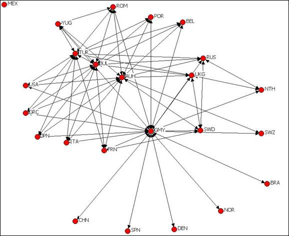
Figure 2: Level of Conflict Network for World War I. (Country names are Correlates of War abbreviations.)
Compare Figure 2 with the list of the
blocks in World War I in Table 4.
|
Allies (Entente) |
Central Powers |
Neutrals |
|
|
|
|
|
|
|
|
|
|
|
|
|
|
|
|
|
|
|
|
|
|
|
|
|
|
|
|
|
|
|
|
|
|
|
|
|
|
|
|
|
|
|
|
|
Balkans (YUG) |
|
|
Table 4: Conflict Blocs in World War I
The
Central Powers in the middle of Figure 2 are not linked by conflict ties with
one another (except for something between
(insert the graphic of trade network in
1880 here and compare it with the next figure)
Figure
3 shows the network structure of trade in 1913 just before the outbreak of
World War I. The cutting point we used for the trade network graphic is
______________.
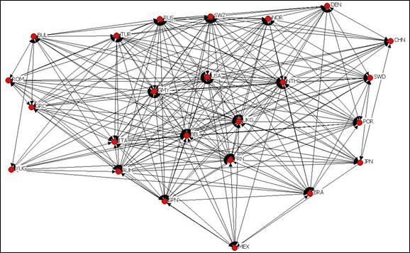
Figure 3 Trade Network for 1913. (Country names are the Correlates of War abbreviation.)
The
trade network graphic uses the values for dyads that we used in our
correlational analysis above. We have trade networks every five years from
1880 to 1913. This is a dense network but it clearly has a multicentered core
and a periphery.
Multiplicative Coreness
The
interaction matrices were also used to calculate multiplicative coreness. A multiplicative core
is characterized as a set of nodes possessing a high density of connections
amongst themselves, while the multiplicative periphery is characterized as
possessing few interconnections. The
consequence of such a structural condition is that nodes located within the
core are often capable of greater coordinated action and a greater
mobilization of resources, while nodes in the periphery are not. Computed a
coreness score for each country using the trade matrices for every five years
between 1880 and 1913 and then used these score to compute a gini coefficient
that indicates how much dispersion there is in the distribution of coreness
scores across countries.
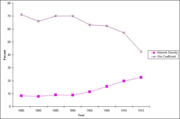
Figure 4 Graph of the relationship between the Gini Coefficient and Level of Network Density for the Trade Network from 1880 to 1913
Figure 4 is the graph
demonstrating the relationship between the Gini Coefficient and the Level of
Network Density for the Trade Network of participants in World War 1. In network analysis, Gini Coefficient
measures the amount of inequality between the core and periphery nodes in
terms of the distribution of connections. (What is network density?) Within the trade network presented here the
level of inequality as indicated by the Gini Coefficient declines slightly
from 1880 to 1910 and then it declines steeply. This indicates that the
network is becoming less centralized as British hegemony in the world economy
is declining because other countries are growing. From 1880 to 1910 the core of the network
consists solely of the
At the same time the
Gini Coefficient is decreasing, the density of the network is increasing. In other words, the centralization of control
over trade in the world-system is decreasing at the same time the level of
competition for trade is increasing. Thus at the level of the global economy,
a clear increase in the level of competition and distribution of resources
preceded the world war, and these changes accelerated in the years just before
the outbreak of the war. [7]

Table 5: QAP correlations between the level of trade between nodes in the network and the level of conflict occurring during World War 1
We used
the QAP routine in UCINet to produce Pearson’s r correlation coefficients for
the values in the square conflict and trade matrices. QAP assesses the frequency of
random correlations as large as those actually observed, making it possible to
test the statistical significance of the observed correlations between two
square matrices despite the fact that the cells are not independent from one
another.
As was the case in the dyadic analysis, there is a clear non-negative correlation between trade and conflict. In other words, the more the nodes of the network trade with each other, the more likely they are to go to war. Unlike the dyadic analysis though, only the levels of trade in 1913 and 1910 are significant predictors of the level of conflict in World War 1. Interestingly, the size of the positive correlations is the same for both the dyadic and network analysis.
We used UCINet’s Faction routine to identify trade factions from the trade network matrix. The Faction routine allows valued data but requires specification of the number of factions. When three factions are specified UCINet groups the countries as shown in Table 6 based on the trade network data. Table 6 also shows which countries are in which conflict bloc.
|
Entente Allies |
Central Powers |
Neutral |
|
|
|
|
|
Belgium 2 |
Austria-Hungary 2 |
Brazil 1 |
|
France 2 |
Bulgaria 2 |
China 3 |
|
Greece 2 |
Germany 1 |
Denmark 1 |
|
Italy 3 |
Turkey 2 |
Mexico 3 |
|
Japan 3 |
|
Netherlands 1 |
|
Portugal 1 |
|
Norway 1 |
|
Romania 2 |
|
Spain 1 |
|
Russia 2 |
|
Sweden 1 |
|
UK 2 |
|
Switzerland 1 |
|
USA 3 |
|
|
|
Balkans 2 |
|
|
Table 6: War Factions and Trade Faction (1,2, and 3)
Table 7 below is a crosstabulation of the conflict blocs and the trade factions.
|
|
|
War faction |
|
|
Total |
| |
|
Entente Allies |
Central Powers |
Neutrals |
|
|
Trade faction #1 |
1 |
1 |
7 |
9 |
|
| |
Trade faction #2 |
7 |
3 |
|
10 |
| |
Trade faction #3 |
3 |
|
2 |
5 |
| Total |
|
11 |
4 |
9 |
24 |
For the Entente
Allies 7 of 11 are in trade faction #2. For the Central Powers 3 of 4 are
also in trade faction #2. For the Nuetrals 7 of 9 are in trade faction #1.
None of the Central Powers are in trade faction #3, which contains 3 Entente Allies
and 2 Neutrals.
So there is not a great match
between the trade factions and the conflict blocs. Trade faction #2 contains
75% of the Central Powers and 64% of the Allies. The best match is
that 7 of 9 Neutrals are in trade faction #1. It would seem logical
according to the liberal hypothesis that a country would remain neutral if it
was trading with both sides and did not want to offend either one. But
instead Tables 6 and 7 show that those countries that were less connected
with either side by trade were more likely to remain nuetral. And
Thus the
results of network analysis do not contradict earlier findings or the
replicated (and improved) dyad analysis described above. Indeed there is some
additional positive support for the notion that trade connections do not
reduce the likelihood of conflict. But a new connection between trade and
conflict is shown in Figure 4 above. The overall shape of the trade network
was changing in the decades prior to the war and these changes accelerated
just before the war. The network was getting denser and less hierarchical.
The centrality of
The lack
of correspondence that we find between trading factions and the conflict
blocs that emerged in the Great War echos what many war historians have often
said – the structure of alliances were fluid and did not gell until just
before the conflagration. As late as 1901, during the second Boer War, the
populations of both
References
Alderson, Arthur S. and
Jason Beckfiled 2004 “Power and position in the world city system,”
American Journal of Sociology 109:811-51.
Arrighi, Giovanni 1994 The Long Twentieth Century.
Bairoch, Paul and
Richard Kozul-Wright 1998 “Globalization myths: some historical
reflections on
integration, industrialization and growth in the world economy,”
pp. 37-68 in Richard
Kozul-Wright and Robert Rowthorn (eds.) Transnational
Corporations and the Global Economy.
Barbieri, Katherine
2002 The Liberal Illusion: Does
Trade Promote Peace?
Barr, Kenneth, Shoon
Lio, Christopher Schmitt, Anders Carlson, Kirk Lawrence, Jonathan
Krause, Yvonne Hsu, Christopher Chase-Dunn and Thomas
E. Reifer 2006 “Global
conflict and elite integration in the 19th and early 20th centuries” Presented at the
Annual
Meeting of the American Sociological Association, in
at 10:30 am on August 11, 2006 at the session on World Systems organized by
Farshad
Araghi. IROWS Working Paper
#27 available at https://irows.ucr.edu/papers/irows27/irows27.htm
Bollen, Kenneth A. 1989
Structural Equations with Latent Variables.
Bornschier,
Volker and Christopher Chase-Dunn (eds.) 1999 The
Future of Global Conflict
Carroll, William K.
Forthcoming “Global cities in the global corporate network” American
Journal
of Sociology.
Carroll, William K. and
Colin Carson 2003 “The Network of Global Corporations and
Policy Groups: A Structure for Transnational Capitalist
Class Formation?” Global
Networks
3 (1): 29-57.
Chase-Dunn, Christopher 1990 “World State Necessity” Political Geography Quarterly, 9,2: 108-30 (April). https://irows.ucr.edu/papers/irows1.txt
Chase-Dunn, Christopher
2005 “Upward sweeps in the historical evolution of world-
systems” IROWS Working Paper #20 available at
https://irows.ucr.edu/papers/irows20/irows20.htm
Chase-Dunn,
Christopher, Yukio Kawano and Benjamin Brewer 2000 "Trade
Globalization since 1795: waves of integration in the world-system,"
American Sociological Review
65:77-95 (February). summarized in Scientific
American June 2003.
Chase-Dunn,
Christopher, Andrew Jorgenson, Rebecca
Giem, Shoon Lio, Thomas E. Reifer and John Rogers, 2002 “Waves of Structural
Globalization since 1800: New results on Investment Globalization”
A paper presented at the annual meeting of the American Sociological Association,
August 16-19, Chicago.
Chase-Dunn,
Christopher, Andrew Jorgenson, Shoon
Lio and Thomas Reifer, 2005
"The Trajectory of the
United States in the World-System: A Quantitative Reflection"
Sociological Perspectives.
Choucri, Nazli and
Robert North 19xx Nations In Conflict.
Eugene Date Management
Software: www.eugenesoftware.org
Freeman, Linton C.,
Douglas R. White and A. Kimball Romney 1992 Research Methods in Social Network Analysis. Transaction Press
Goldfrank, Walter L.
1977 “Who rules the world: class formation at the international level” Quarterly Journal of Ideology 1,
____________1983 “The
limits of an analogy: hegemonic decline in
the
Hanneman, Robert nd Introduction to Social Network Methods
http://faculty.ucr.edu/%7Ehanneman/SOC157/TEXT/TextIndex.html
Held, David, Anthony
McGrew, David Goldblatt and Jonathan Perraton. 1999. Global Transformations:
Politics, Economics and Culture.
Hirschman,
Albert O. 1980 [1945] National Power
and the Structure of Foreign Trade.
Johnson, Ian 2000 “A
step-by-step guide to setting up a TimeMap dataset.” Archaeological
Computing Laboratory.
Junne,
Gerd 1999 “Global cooperation or rival trade blocs?” in Volker Bornschier and
Christopher Chase-Dunn (eds.)
The
Future of Global Conflict.
.
Kentor, Jeffrey. 2000a.
“Shifting Patterns of Organizational Control in the World-Economy 1800 1990.”
Funded Grant Proposal
to World Society Foundation:
_____. 2000b. Capital and Coercion: The Economic and
Military Processes That Have Shaped the World Economy 1800-1990.
Kentor, Jeffery and
Yong Suk Jang 2004 “Yes, there is a transnational business community.” International Sociology 19,3:352-368.
Korzeniewicz, Roberto
Patricio, Angela Stach and Vrushali Patil 2004 “Measruing national income: a
critical assessment.”
Comparative Studies in Society and History
Krasner, Stephen D.
1976 “State power and the structure of international trade,” World Politics 28,3:317-47.
Kravis, Irving B., Alan
Heston and Robert Summers 1982 World
Product and Income:
International Comparisons of Real Gross Product.
University Press.
Krempel, Lothar
and Thomas Pluemper 1999
“International division of labor and global economic processes:
an analysis of the
international trade in automobiles” Journal
of World-Systems Research, 5,3:487-498
Levy, Jack S. 1983 War in the Modern Great Power System,
1495-1975.
University Press of
Maddison, Angus 1995 Monitoring the World Economy, 1820-1992.
Economic Cooperation
and Development.
_________ 2001 The World Economy: A Millennial
Perspective.
Cooperation and
Development
Mitchell, B.R. 1992 International Historical Statistics:
____________ 1993 International Historical Statistics: The
NY:
____________ 1995 International Historical Statistics: Africa, Asia, &
2nd ed. NY:
Maoz, Zeev 2006. “Network Polarization, Network Interdependence, and International Conflict, 1816-2002.” Journal of Peace Research, 43(4): 391-411 http://jpr.sagepub.com/cgi/reprint/43/4/391 Maoz, Zeev, R. Kuperman, L. Terris, and I. Talmud. 2004 “International Relations: A Network Approach." in New Directions for International Relations, Edited by A. Mintz and B. Russett. Lanham , MD : Lexington Kuperman, and L. Terris). http://soc.haifa.ac.il/~talmud/evolution.pdf Maoz, Zeev, R. Kuperman, L. Terris, and I. Talmud. forthcoming "Structural Equivalence and International Conflict, 1816-2000: A Social Networks Analysis of Dyadic Affinities and Conflict." Journal of Conflict Resolution http://soc.haifa.ac.il/~talmud/strucequiv.pdf Maoz, Zeev, R. Kuperman, L. Terris, and I. Talmud. forthcoming "The Enemy of my Enemy: The Effects of Indirect Enmity Relations on Direct Dyadic Relations," Journal of Politics .
O’Rourke, Kevin H and
Jeffrey G. Williamson 1999 Globalization
and History: The Evolution of
a
19th Century Atlantic Economy.
Polanyi, Karl 2001
[1944] The Great Transformation.
Rasler, Karen A. and
William Thompson. 1994. The Great
Powers and Global Struggle: 1490 1990.
Reifer, Thomas E. 2002
“Globalization & the National Security State Corporate Complex (NSSCC) in
the Long Twentieth Century,”
Reifer, Thomas E. and
Christopher Chase-Dunn 2003 “The Social Foundations of Global Conflict and
Cooperation:
Waves of Globalization
and Global Elite Integration, 19th to 21st Century. Research Proposal Funded
by the National
Science Foundation’s
Sociology Program. https://irows.ucr.edu/research/glbelite/globeliteprop03.htm
Reifer, Thomas E.
“Globalization, Democratization & Global Elite Formation in Hegemonic
Cycles: A Geopolitical Economy,”
2005, in Jonathan
Friedman & Christopher Chase-Dunn, eds., Hegemonic Declines, forthcoming
Paradigm Publishers, Ch. 7, pp. 183-201.
Robinson, William I.
2004 A Theory of Global Capitalism.
Rosecrance, R. 1963. Action
and Reaction in World Politics.
Rosecrance, Richard and
Peter Thompson 2003 “Trade, foreign investment and security,” Annual Review of Political Science
6:377-98.
Sklair, Leslie. 2001. The Transnational Capitalist Class.
Smith, David A. and
Douglas R. White 1992 “Structure and Dynamics of the Global
Economy: Network
Analysis of International Trade 1965-1980,” Social Forces 70:857-
894
Sassen, Saskia 2001 The Global City:
Press.
Sklair, Leslie 2001 The Transnational Capitalist Class.
Smith, David A. and
Michael Timberlake. 2001. “
1977-1997: An Empirical
Analysis of Global Air Travel Links.” American
Behavioral
Scientist 44, 10: 1656-1678.
Snyder, Jack 1991. Myths of Empire: Domestic Politics and International
Ambition.
_____. 2000. From Voting
to Violence: Democratization and
Nationalist Conflict.
_____.2003."Imperial
Temptations." The National Interest. 71:29-40.
Su, Tieting. 1995.
"Changes in World Trade Networks: 1938, 1960, 1990" Review XVIII, 3
:431-459 (Summer)
Van der Pijl, Kees.
1984. The Making of an
______________ 1998 Transnational Classes and International
Relations,
Weber, Max. 1961. General Economic History,
Appendix
Histogram
for Level of Conflict Index
Supplementary
Trade Data
According to Barbieri (2003), “The
Statesman’s Yearbook contains country profiles that usually include
tables of foreign trade figures. When
these tables are not present, information was pieced together by reading
entries related to a particular state’s economic activities. For the period 1873-1885 U.S. Congressional
records proved to be a useful source of trade data, in particular U.S.
Congress (House) Miscellaneous Documents (1887), “Abstract of the Foreign
Commerce of Europe, Australia, Asia and Africa, 1873-1885,” United States
Consular Reports, No. 85, October. (
According to Barbieri (2003), “several problems arose
when converting trade figures from local currencies to US dollars. The primary problem was the lack of available
exchange rates for many states. In
many instances trade data reports were available, but exchange rates were
unavailable. In addition, Polity II
contains a variable that lists the name of the national currency to which the
exchange rate is presumed to correspond.
However, in many instances no currency name is given. Also, in some instances, particularly in
Latin American states, the value of import and export flows are reported in
two different currencies. For example,
silver pesos may be used for imports, while gold pesos are used for
exports. This requires separate
exchange rates for converting imports and exports into US dollar values (see
Appendix for supplementary data sources).”
Links
to Related Data Online
Conflict Data Sets: http://www.pcr.uu.se/pdf/conflictdataset2.pdf
http://www.umich.edu/~cowproj/dataset.html
(Link to Correlates of War Project; includes a number of datasets that deal
with war/conflict)
Katherine Barbieri
Trade Data Sets:
http://sitemason.vanderbilt.edu/site/k5vj7G/new_page_builder_4
http://weber.ucsd.edu/~kgledits/Polity.html
(Link to POLITY project datasets, which include data on cross-national
authority structures)